Sunday, November 10, 2013

Go-ogle map-delbrot

Go-ogle Map-delbrot

In a previous post I looked at using Python to write a mandelbrot server that could be used as a custom source in google maps.

I thought I'd try to do the same using Go.

It starts by defining some structures for mandelbrot requests. I separate the request and the description structures so that when we can cache the data based only on the description. Note that the mand_request has a mand_desc anonymous field, which allows us to transparently access the mand_desc fields from a mand_request.

type mand_desc struct{
 w, h int
 max_it int
 sx, ex, sy, ey float64 
}

type mand_request struct{
 mand_desc
 out io.Writer
 donechan chan int
}

We then create a channel that accepts a mand_requests, we'll be pushing requests to this later:

var mand_request_channel = make(chan mand_request)

We'll store calculated images in a cache (a map of Image.Palletted pointers (an object from the default Image package) keyed by a mand_desc object):

var cache = map[mand_desc] *image.Paletted {}

To enable concurrent processing we have to explicitly set the runtime.GOMAXPROCS variable. We set it to the number of CPUs in the system, and start a goroutine for each one:

runtime.GOMAXPROCS(runtime.NumCPU())
for i := 0; i < runtime.NumCPU(); i++ {
 go mand_handler(mand_request_channel)
}

The mand_handler function waits for a request and creates the mandelbrot or uses the previously cached version. Then we encode the data and write it to the io.writer in the mand_request. Finally we put a value into the donechan just to indicate we've finished.

func mand_handler(inchannel chan mand_request) {
 for m := range(inchannel) {
  ret, ok := cache[m.mand_desc]
  if !ok{
   ret = make_mand(m.w, m.h, m.max_it, m.sx, m.ex, m.sy, m.ey)
   cache[m.mand_desc] = ret
  } else {
   fmt.Println("Hitting cache!")
  }
  png.Encode(m.out, ret)
  m.donechan <- 1
 }
}

The rest of the code sets up the HTTP server and creates the mandellbrot image. The full code can be found on GitHub.

Go and Python


Comparing the two versions, there's probably more in common than there are differences. Both rely on libraries to do a lot of the hard work (HTTP server, png compression) but in fact the Go program used only standard libraries, whereas Python needed numpy and matplotlib (which admittedly are so common as to almost be standard).

Speed Comparison


Although Go is compiled, and a lot closer to the hardware then Python, I was expecting the two to be a similar speed - most of the time is spent in squaring and adding complex numbers, which numpy does in compiled code anyway. The Python code is fundamentally less efficient in a few ways: 
  • It still squares and add pixels that have already diverged whereas the Go code moves onto the next pixel immediately
  • I'm using the numpy abs function to see if the pixels have diverged, which has a square root per pixel (the go version compares x^2 to limit^2 instead - it would be possible to do this in Python at the expense of readability)
  • The Python version has to iterate through all pixels once per iteration. The Go version deals with one pixel at a time for all iterations. This is probably faster, as it can keep the pixel data in the cache over the iterations. Maybe.
So having said all that, here's the results (for requesting 100 images, serially):
LanguageTime (s)
Go3.1
Python21.9

Here we can see just how much faster (surprisingly to me) the Go code is. I tried replacing the np.abs(m)>2 call with np.real(m*m.conjugate())>4 instead (saving a square root, but needing to go in and out of Python more times) and it slowed things down by about 10%. So Go is significantly faster than Python in this case.

Final Thoughts


After playing with Python for a while, it's nice to return to a compiled language to see just how fast things can be. The nice features of Go are the extensive standard libraries, the speed, and the goroutine and channel philosophy. It doesn't have anywhere near the number of third-party libraries that Python has however. Go feels like a lean (it's closer to C than C++), fast language with a small number of really helpful higher level abstractions (channels, maps, slices) combined with very lightweight concurrency (goroutines).


Saturday, September 7, 2013

A-Flat Minor part II - Chords

A-Flat Minor part II—Chords

In the previous post, I discussed chords and how harmonics of a single note can be considered the basis for the notes of a chord. There's a very interesting discussion of how chords relate to the harmonics of a single note in this article originally published in Experimental Musical Instruments (which basically inspired this whole project). One of its claims (if I understand correctly) is that consonance only really occurs between identical notes, and chords themselves only sound consonant because they have shared notes in their harmonics (this means that if we call the harmonics of a single note timbre then we can say that notes of a nice-sounding chord depend only on the timbre of the instrument - the traditional major chord sounds nice only with a timbre that produces harmonics which are exact integer multiples of the root).

Part I looked at the notes in the harmonics, and this part will look at the common frequencies in both major and minor chords.

Major Chords

Previously, we saw how the harmonics of a single note produced a range of other notes. The diagram below shows the notes reached (as indicated by angle on the spiral) by these harmonics:


The notes for the major chord are taken from the first three unique angles encountered, the I, V and III notes.

What happens when we play a major chord using these three notes? The following shows us:


There's a lot of information in this chart, and I'm not sure exactly how to interpret it all. The root (I) and its harmonics are in red, the fifth (V) and its harmonics in blue and the third (III) in green. When notes coincide, the colors are combined additively (as indicated in the key in the top left). The first thing to note is that the III and V notes both combine with the root (turning from green to yellow and blue to magenta respectively). This isn't surprising, as we picked those notes exactly because of this property. What is maybe more surprising is the lack of white notes, with VII and IV# being the only notes where harmonics from all three notes combine. The II note has combined harmonics from the root and fifth, much like the V itself. Also oddly, none of the other notes have the root (I) as a harmonic, it stays purely red all the way to the edge of the spiral.

Whether our ears actually pick up all this information is another matter, but nonetheless it offers an interesting visual representation of a major chord.

Minor Chords

The Otonality and Utonality link mentioned last time provides an elegant explanation for the notes of a major chord, being the first individual notes from the harmonics of the root, as we saw above. It also provides a similar explanation for the minor chord, with a few adjustments: the notes of a minor chord can be found from the subharmonics of the fifth of a minor chord! The subharmonics are integer divisions of the root frequency, eg  f, f/2, f/3, f/4...  (while the harmonics are integer multiples, eg f, 2f, 3f, 4f... ). If we look for the first unique notes, they are f, f/3, f/5 and again we can multiply by powers of 2 to get them in the same octave. Then we get ratios 1:4/3:8/5 or 15:20:24. Looking at Wikipedia
we see this should be 10:12:15, which we will get if we raise what we've considered the root to the next octave (and stick it on the end) giving us 20:24:30 = 10:12:15.

So what's going on here is that a minor chord is composed of the I, IIIb, V notes , and we can justify this by saying the notes are the first sub-harmonics of the V note. [Because I'm such a fan of this elegant theory, if it was up to me I'd prefer to rename minor chords to use the fifth rather than the root as the identifier - I'm guessing the reason the current scheme is used is due to the similarity to the major chord eg I, III, V for the major vs I, IIIb, V for the minor (you just have to move one finger on a piano!). If the fifth was the root, the notes would be I, IV, VIb which means moving two fingers!] I'm going to use both chords below, referring to the I, IV, VIb chord as a 'pseudo-minor' chord

All this theory about the minor chord is actually a lot easier to see in the diagram of the harmonics:


The above is the harmonics of the pseudo-minor. The I, IV and VIb notes are the first three notes that have a harmonic at the I position (we can see this clearly here, the 12 o'clock notes turn from red to yello to white as the harmonics combine). We can also see white notes on the III and V positions (even though the V note is not one of the chord notes it seems to play a significant role). This is in contrast to the major note, where there were relativley few white notes, but a lot more cyan, yellow and magenta notes.

We can look at the more traditional minor chord too:


This is essentially the same as the previous diagram, but rearranged so that what was the IV note (all green in the previous diagram) is now rotated to the root (red), and the old root is increased by an octave and is now at the 6 o'clock V position (and blue). Again we see all three notes having harmonics at the V position (instead of the root) and white notes at the II position (which was V previously!).

More Notes?

I'm really pleased with the way these diagrams have turned out. If you want to play with the source and try to see what other chords look like, it's available on Github (it needs the ui_decorators class and PySide for the UI to work). There's lots to think about here, but two things I find interesting: The lack of a note at the 9 o'clock position, it has strong harmonics from the root (and even the IV note in the pseudo minor) and the number of harmonics found at the II and VII notes (especailly the VII note - it has harmonics from all notes in bot the major and minor chords). I haven't looked at what happens if we add a VII note to the mix, mainly because things seem complicated enough, and we're starting to run out of colors.

Another thing worth mentioning is that although the Python program can play the notes it creates, I've been mostly using it with the sound turned off. It may be there's not enough variation in the frequencies, but either way the actual notes sound pretty harsh and not particularly pleasant - I think it works better as a visual aid rather than an aural one.

More Pictures

The diagrams above have been starting at 440Hz and stopping at 22.1kHz, giving around 6 octaves or so. These limits were chosen as a sensible starting frequency and then a sensible upper limit for the human ear. However, we can choose to increase these limits and get more octaves. I'm including some more pictures here starting at 64Hz instead, giving us another few octaves, and at a higher resolution (1200x1200 instead of 600x600). The notes are smaller so they don't arbitrarily overlap at the higher octaves.


Major Chord


Minor Chord


Pseudo-minor Chord


A-Flat Minor part I - Harmonics

A-flat Minor I—Visualizing harmonics

What is a major chord? It sounds like a simple question, and if you ask a musician, they might say something like a root, a major-third and a prefect fifth. When I started looking into chords and how they're created this seemed like a great answer. Surely these fractions correspond to some perfect ratios, where a third indicates maybe a third of the main frequency and a fifth is a fifth Or at least something to do with 3 and 5. Erm, no. It turns out you simply count, starting at 1: a 'third' is simply the third note you reach and the fifth the fifth (eg for the scale of C, a 'third' is E and a fifth is G, you just count up from C, with C=1).

So in that case, what is a major chord? Wikipedia comes to the rescue, telling you it's notes in the ratio 4:5:6. This is at least meaningful, but seems a little arbitrary - how are these ratios chosen and why do they sound so good together? Luckily, there's a link from there to a very interesting page about Otonality and Utonality. Here, it describes how the major chord can be made up of the first three unique notes from the integer harmonics of a note (ie for a note with frequency f, we take 2f, 3f, 4f... etc., these tend to happen to some extent in real instruments naturally). Let's take C4 (middle C, 262.626Hz) as an example, and look at the notes we get for the first few harmonics:

NoteHarmonic
C41
C52
G53
C64
E65
G66
A#6 (ish)7
C78

Here we can see the first 3 unique notes (C4, G5, E6) have ratios of 1:3:5. However, because doubling (or halving) the frequency gives us the same note, we can move the notes to the same octave by multiplying by 4, 2,1 to  give us the 4:6:5 ratio we expect. (It might seem odd that a major chord has no notes above 6/4 times the root note. What happens to the next obvious choice: 7/4? I think this note gets too 'close' to the root note (in linear scale, both 5/4 and 7/4 are 1/4 away from the root, but acoustically I think the 7/4 (or 7/8 if we move it to just below the root) starts to sound very close to it and a little discordant. Maybe.)

Visualizing Harmonics

Is there a simple way to visualize these harmonics? What would be nice is a way to see harmonics and get some idea of the note and octave. A common way of visualizing this is using a music helix where the note becomes an angle and the octave a height. This can then be flattened to form a spiral (and there's a fascinating website about that here, with a lot of videos of music and the corresponding spectrogram).

I used Python to write a program that would allow me to visualize harmonics and chords in a similar fashion. Here's what a single root note, with no harmonics looks like:


The small red bar near the center represents the root note. As more notes get added, they'll appear on the spiral, further out at higher frequencies and at an angle corresponding to the note.

Now lets look at the first 3 harmonics:


We again see the root, red, and right above it the second harmonic in green. The third harmonic appears further along on the spiral in the fifth (V) location in blue. The third harmonic is the 'fifth' mentioned earlier (ie G if the root is C).

Now let's look at the first 5 harmonics, and see the notes of our major chord:


This time the first, second and 4th harmonics are in red (they're all the root note, say C), the 3rd in green (this is the V, G) and the 5th in blue (the 'major third', III, E). These are the three notes of the major chord, represented here with the root at 12 o'clock, the 'fifth' at 6 o'clock and the major third at 3 o'clock.

It's interesting to see what notes we hit if we just keep adding harmonics. What happens if we just add harmonics up to an arbitrary limit? Below I start at 440Hz and add all harmonics til we reach past the limit of most people's hearing, 22.1kHz:


Here we can see that once a note has been hit, it will get hit again the next go round (not surprisingly, as if h is a harmonic, so will 2h). It's also interesting to see which notes in the scale we hit - after the III and V notes, we hit the II and VII notes pretty early on, and then some odd incidentals (IIb and IV#). Oddly, the 7th harmonic (9 o'clock in the diagram above) isn't close to any of the natural notes, even though it's the next unique note after the major chord notes. (This is arguably a case for dismissing harmonics much higher than the 7th - after all, if the 7th harmonic is the next one and we haven't even bothered naming a note for it, can harmonics any higher than this really be that important? I'm going to ignore that question and carry on ignorantly).

I'm going to stop there and next time look at what happens when you combine the harmonics of the chords together, and also take a look at minor chords. You can find part II here.

Technical details about the charts above

In the charts above, I've decided to make the angle linear with frequency so that the fifth, which is 3/2 the root, occurs at 180 degrees. This means that doubling the frequency of a note will some of the time put the note 180 degrees opposite, and sometimes not. If I had used a log scale for the notes, a doubling would be the same for all the notes, but at a rather less convenient 210 degrees. The software below allows you to choose either method. The lines for the notes are for the just intonation tones.

Software

The software used to create the diagrams above is available from my github account. The UI requires the ui_decorators module, talked about here.


Monday, July 29, 2013

Prototyping UI in Python

Prototyping UI in Python

I like Python, but I don't like typing. Ever since starting to play around with Python, I've found it easier to write and test programs (running individual modules easily is a really nice feature, and skipping the whole compile step just seems, maybe psychologically, quicker and simpler).

But, paradoxically (or maybe not), I've found myself typing a lot more. I start up python, import a module, make a few object, call some functions etc, invariably find a bug, try to fix it and then repeat the whole process again. If I was using, say, C#, I'd probably have to write some extra UI code, hook up a function to do all the above to a button or menu item, then run the whole program, just to test that bit. It would be less flexible, as I'd have to recompile everytime I wanted to change the test function, but it means I just have to click a single button (or menu item) to test - no typing required.

So why not use a similar approach in python? Write a test function, and hook it up to a button somewhere? There's plenty of UI options to choose from (I've dabbled in TkInter, WxPython and Qt). Personally, I find they all seem to get in the way a bit. Your main function ends up being modified to run an application loop, you need to remember the names of the widgets you want, there's all kinds of advanced options for things I don't need, I just want a button! (I find Qt especially bad in this respect, mainly because Qt is no longer a UI framework, but rather an application framework. If you're willing to use QObjects and QLists and QTime and QInt etc, instead of the language standards, you're fine. Otherwise you need something to convert your model into a Qt compatible model (could this be a new model-qtmodel-qtcontroller-uimodel-uicontroller pattern??))

Ideally, this is what I'd like:

class A:
    @button
    def func1(self):
        ...

a=A()
ui_display(A)

I don't care how the button looks, what color it is, how big it is (as long as I can read the text) or even which framework gets used. I'm happy for it to display the name of the function, and for the ui_display function to hog the main thread til I've dismissed it.

There are two parts to solving this problem: First, how to decorate functions in a framework-independent way, and secondly, how to convert an object with decorated functions into a framework specific UI. It ended up being a little more complicated than the version above, but also a little more featured (eg, set functions update the ui automatically).

(TraitsUI attempts to solve a similar problem. TraitsUI has a far larger scope (eg using Traits to describe types of variables, etc) and a lot more functionality, what's below is a lot simpler, and uses more standard python code)

UI Decorators

The example above of a button decorator is a very simple case: A button has no state to it, it's clicked once and we expect an event to happen once. But how about something like a slider or text box? In this case we have more constraints: The slider has a state (the position of the cursor along the slider) that we want to be kept in sync with the object state. We can achieve this by decorating a set function, and then making sure the slider gets updated every time it's called. There's also the case of finding the state of the object at the time the slider is created. In this case we don't want to rely on waiting for a call to the set function, so instead we supply an optional get function to the decorator.

The decorator for creating a slider ends up looking like:

class Test:
    @slider(getfunc=get_test)
    def test(self, newval):
        ...

    def get_test(self):
        ...
        return number

Internally, all the decorator is doing is adding some attributes to the function: a _slider dictionary with information about the decorator, and a (fake) instance method
listeners, which returns the listeners for the function for the object specified. Eg:

>>> t=Test()
>>> t.get_test.slider
>>> t.test._slider
{'getfunc': , 'scale': 1, 'minimum': 0, 'maximum': 100}
>>> t.test.listeners(t)
[]
>>>

Currently, there's similar decorators for combobox, checkbox, textbox and button. The decorators are designed to be mostly side-effect free, so using them in a case when you don't end up using a UI shouldn't cause any major problems (there's an extra dictionary per function per class, and an extra list per function per instance).

UI Frameworks

To actually use the decorators, there needs to be a framework module to convert a class with decorated functions into a UI object. It supplies a function get_obj_widget, which returns a UI-specific widget for a decorated object, and display_widgets, which displays the given list of widgets (either created via get_obj_widget, or some other means). A helper function, display, calls these in succession, creating and displaying the given object.

Currently only a (PySide-based) Qt framework exists. The widgets created are DockWidgets, and can be moved around and docked independently.

I've written this specifically for another project I was playing around with, I'll post that next.

You can find the files on Github. ui_decorators.py has a little sample application if run as the main module, it requires PySide.

Tuesday, April 23, 2013

GoogleMap-delbrot

Google Maps, Python and the Mandelbrot Set

There's some surprising uses for a Mandelbrot set (or similar fractal). With just a small bit of code (and a little bit of computation), you can create an image that has detail at any level, and has varied features over the image so its possible to tell where you are. I've used this at work when debugging a scan system that could scan with fields-of-view from 2000nm to 1nm. It also had the ability to scan sections of the image. By writing a Mandelbrot generator as a test scan unit, I could test all of this functionality (I even had the number of iterations tied to the scan pixel time).

I was recently looking at creating a custom Google map, and I thought that using the Google Maps API to browse a Mandelbrot set might be pretty sweet.

It seems other people have had similar ideas, there's a version here and here, although I couldn't find the source for the first one, and the second doesn't include the continuous-zoom feature that Google maps has. This version only runs locally and needs Python for the webserver, and a browser for viewing the final page.

Creating the Mandelbrot Set

I wanted to use Python to create the Mandelbrot set and serve it locally. I split it into two files, one that creates a Mandelbrot set for a given set of coordinates, and another to respond to HTTP requests and return the requested image.

Creating the Mandelbrot set is relatively easy in Python, although a little different than I'd normally do so. Because whole-image operations are optimized in Python, it's faster to use them to create the set rather than iterate over each pixel individually (this also means that we don't escape from the algorithm once a pixel has diverged, we continue to process it for further iterations). I used a slightly modified version of the code from the scipy website, shown below:

#mandelbrot.py
#creates a mandelbrot for the given coordinates
import numpy as np

def mand(iters, tl, br, xpx, ypx=None):
    ypx = ypx or xpx
    c=np.add(*np.ogrid[tl[0]*1j:br[0]*1j:xpx*1j,
                       tl[1]   :br[1]   :ypx*1j])
    m=c.copy()
    ret=np.ones(c.shape, dtype=np.int32)
    for it in xrange(iters):
        m *= m
        m += c
        ret += np.abs(m) < 2
    #want inf. iterations to be a single color, not based on # of iterations
    ret += -(iters+1)*(np.abs(m) < 2)
    return ret

def mand_and_write(file, iters, tl, br, xpx, ypx=None):
    from matplotlib import pyplot
    m=mand(iters, tl, br, xpx, ypx)
    pyplot.imsave(file, m, cmap='spectral', vmin=0, vmax=255)
    
if __name__=="__main__":
    from matplotlib import pyplot
    m=mand(16, (-2, -2), (2, 2), 256)
    pyplot.imshow(m, cmap='spectral') 
    pyplot.show()

If you run this on it's own, it should show a small 256x256 Mandelbrot set:

The next step is to create the webserver, and route requests to our Mandelbrot generator. I decided to just split the request using '/'s, so a GET request with a path of /-2/-2/2/2/16 returns a 256x256 png from (-2,-2) to (2,2) with 16 iterations. The code is below:

#mandserver.py
#simple amnd server that returns pngs for a mandelbrot
from BaseHTTPServer import BaseHTTPRequestHandler, HTTPServer
import mandelbrot
use_threaded_server = True
if use_threaded_server:
    from SocketServer import ThreadingMixIn

import cStringIO


class MandServer(BaseHTTPRequestHandler):
    cache = {}

    def do_GET(self):
        self.send_response(200)
        self.send_header("content-type", "image/png")
        self.end_headers()
        #we'll skip the leading slash
        if self.path not in self.cache:
            coords = self.path[1:].split('/')
            print self.path
            start = -1, -1
            end = 1, 1
            iters = 16
            if len(coords) >= 2:
                start = float(coords[0]), float(coords[1])
            if len(coords) >= 4:
                end = float(coords[2]), float(coords[3])
            if len(coords) >= 5:
                iters = int(coords[4])
            print "requesting ", iters, start, end
            memFile = cStringIO.StringIO()
            mandelbrot.mand_and_write(memFile, iters, start, end, 256)
            self.cache[self.path] = memFile
        else:
            print "Hitting cache!"
            memFile = self.cache[self.path]
        memFile.seek(0)
        self.wfile.write(memFile.read())


def main():
    httpserverclass = HTTPServer
    if use_threaded_server:
        class ThreadedHTTPServer(ThreadingMixIn, HTTPServer):
            pass
        httpserverclass = ThreadedHTTPServer

    try:
        server = httpserverclass(('', 8080), MandServer)
        print 'started MandServer...'
        server.serve_forever()

    except KeyboardInterrupt:
        print '^C received, shutting down server'
        server.socket.close()

if __name__ == '__main__':
    main()


If you run this, with mandelbrot.py from above in the same folder, it should start serving up the PNGs. You can test it (locally) by going to http://localhost:8080/-2/-2/2/2/16 and confirming you see an image similar to the one above (with a slightly different color scheme). The wbeserver runs threaded, so there's a new thread per request. Images are cached as they're created, so if you run this for a long time in can build up a big cache of viewed images.

Now we just need to get Google Maps to request images from this local address in the right format.

Custom Google Map Source

The first step to creating a custom Google Maps source is getting an API Key. You can do that here. Make sure that the 'Google Maps API v3' service is turned on in the 'Services' tab. Then copy your personal API key from the 'API Access' window.

Actually creating the custom map is relatively easy. We need to create a google.maps.ImageMapType that takes a structure containing the URL to request from and some other options, like the maximum zoom size (we use the highest, 19). I decided to automatically increase the iteration count as the zoom increases. The html is below, make sure to replace %Your-API-Key% with your API Key (surprise):

<!DOCTYPE html>
<html>
  <head>
    <meta name="viewport" content="initial-scale=1.0, user-scalable=no" />
    <style type="text/css">
      html { height: 100% }
      body { height: 100%; margin: 0; padding: 0 }
      #map_canvas { height: 100% }
    </style>
    <script type="text/javascript"
      src="http://maps.googleapis.com/maps/api/js?key=%Your-API-Key%&sensor=false">
    </script>
    <script type="text/javascript">

var mandelbrotTypeOptions = {
  getTileUrl: function(coord, zoom) {
      var bound = Math.pow(2, zoom);
 var left=(coord.y/bound - 0.5)
 var top= (coord.x/bound - 0.5)
      return "http://localhost:8080/" +  left +
      "/" + top +
      "/" + (left + 1.0/bound) +
      "/" + (top  + 1.0/bound) +
      "/" + (32*(zoom+1));
  },
  tileSize: new google.maps.Size(256, 256),
  maxZoom: 19,
  minZoom: 0,
  radius: 2,
  name: "Mandelbrot"
};

var mandelbrotMapType = new google.maps.ImageMapType(mandelbrotTypeOptions);

function initialize() {
  var myLatlng = new google.maps.LatLng(0, 0);
  var mapOptions = {
    center: myLatlng,
    zoom: 1,
    streetViewControl: false,
    mapTypeControlOptions: {
      mapTypeIds: ["mandelbrot"]
    }
  };

  var map = new google.maps.Map(document.getElementById("map_canvas"),
      mapOptions);
  map.mapTypes.set('mandelbrot', mandelbrotMapType);
  map.setMapTypeId('mandelbrot');

      }
    </script>
  </head>
  <body onload="initialize()">
    <div id="map_canvas" style="width:100%; height:100%"></div>
  </body>
</html>

And that's it. Just navigate to the webpage and you should see a fully functional Google Maps Mandelbrot set. As mentioned above, the results are cached, so that things should speed up if you look at areas you've previously been to.


You can find all the files above at github.

Saturday, April 13, 2013

Hammer Proficiency

Getting Fluent in New Programming Languages

When I first started to learn Python, I wasn't particularly impressed with it. The problem was that searching for an introduction to Python often led to pages that were an introduction to programming using Python as an introductory language, whereas what I really wanted was an introduction to Python for experienced programmers that told me the things that made it different from, say, C. 

So since I couldn't find the introduction I wanted, I referred to the reference docs. The problem with this approach is that it doesn't really get you fluent in a new language, rather it just allows you to write in a language you already know with a different syntax. I'm going to call this 'hammer proficiency', as in if all you have is a hammer, everything looks like a nail. Basically you've got a new tool, and you've learnt enough about it to hit nails with, but not much else.

Here's an example of being 'hammer proficient' in Python. I'm going to write a function that takes a list of strings and returns another list containing only the strings containing the text 'cat', but doing so from a procedural, C-style viewpoint. I know I'm going to return a list, so I'll look up list creation, and I know I'm going to have to iterate over a list, so I'll look up how to iterate over a range of numbers and to find the length of an array. I'm also going to have to look up how to search for strings in a string and add elements to a list. So I would probably come up with something like:

def filter_cat(strings):
    ret = list()
    for i in range(len(strings)):
        if strings[i].find('cat') != -1:
            ret.append(strings[i])
    return ret

There's nothing fundamentally wrong with this. The problem is that any modern language is likely to be flexible enough that you can write code like this, translating almost line-by-line from a more traditional C-style, procedural approach into the new language. But doing so means you don't get to learn the unique and hopefully advantageous features of the program that you're trying to learn.

If I was to write the same function as above now, after having learnt some more Python, I'd probably do the following, using a lambda expression, a list generator and the 'in' operator:

filter_cat2 = lambda strings: [s for s in strings if 'cat' in s]

Which is now using the features included with Python. Only once you start to know not only the syntax, but also the best approaches to take for a given problem for that language, can you really claim to be fluent.

Getting to Fluency

So, how do you get from hammer proficiency to fluency? Experience (and maybe hammer time?) is obviously one way to get there. I didn't find a wealth of information online answering this problem. Like I said, a lot of the introductory information I found started out from too low a level.

StackOverflow has an (unfortunately closed) list of cool features of Python. There's also a really good list of Python tips and tricks here. Finally, I've been doing a few of the Udacity courses (after taking the Stanford 'Introduction to AI' online class). They vary a bit, but the Peter Norvig classes and lectures are all excellent, and his 'Design of Computer Programs' class is too. And because he's using Python, it's serves as an excellent example of how to use the tool, and not like a hammer.

Tuesday, April 9, 2013

Hilbert Curve in Python and Image Compression

Hilbert Curve in Python

After playing with creating a Hilbert Curve in CFDG, I started thinking about how to implement it in Python.  I wanted a way to do so which was easy to understand and which only needed a small amount of data to describe the process.

I decided to write one rule for one specific generation of the curve, and then rotate that rule 4 times, and then for each of those rules flip them. I decided to use a two-character string to decide the basic shapes. The shape can be one of u, [, n, ] where they represent the orientation of the basic u-shaped curve:


As well as that, I had to include the direction around the shape I was going, either 'a' for anti-clockwise, or 'c' for clockwise. So to draw the shape above starting at the top left, I would call it 'ua': It's in the 'u' orientation, drawing anti-clockwise.

I then had to make a mapping, that for a certain shape, eg 'ua', tells us how to treat that shape when we split it into 4 smaller quadrants. I made the starting shape the key, and the values tuples of (quadrant, newshape) with the quadrants numbered as shown below:


So the mapping for 'ua' to the next generation is:


{'ua': [(0, ']c'), (2, 'ua'), (3, 'ua'), (1, '[c')]}

Now all that's left is to rotate three times, to give the [, n, ], anticlockwise rules, then mirror each of those until we finally have all 8 rules. Once this is done, I wrote a function that takes a square power-of-2 2d array, splits it into quadrants and applys the next rule to each quadrant. I made the function then yield the value of the array at that point, that way it essentially maps a 2d array of values into a list of values taken in order following a hilbert curve. To check it worked I made it us Tkinter to plot the values it was returning. The full code is here (also available on github):

# mfm 18Mar13 Trying to make a generator that returns values
# from a 2d array in a hilbert curve
import numpy


def make_mapping(m):
    """
    Return a dictionary built up of a single mapping m rotated and flipped.
    The keys are 2 character strings where
    the first is one of [,],u,n and the second is either 'a'nticlockwise or
    'c'lockwise. The values are a list of integer, tuple pair which
    specify how to split up the 4 quadrants and which (shape, direction)
    pair to apply to it.
    The quadrants are
    ---------
    | 0 | 1 |
    ---------
    | 2 | 3 |
    ---------
    """
    quads = [0, 1, 3, 2]  # quadrants in clockwise order
    shapes = ['u', '[', 'n', ']']  # shapes rotated clockwise
    rots = ['a', 'c']  # possible rotations

    def next(item, list, pos=1):
        """
        Given a list and an item, reurns the item in the list
        pos places after the item.
        Wraps around the list at the boundaries
        """
        return list[(list.index(item) + pos) % len(list)]

    other_direction = lambda x: next(x, rots)
    next_quadrant = lambda x: next(x, quads)
    next_shape = lambda x: next(x, shapes)

    def rotate(key):
        rotated_value = [(next_quadrant(quad), next_shape(shape) + dirn)
                         for quad, (shape, dirn) in m[key]]
        shape, dirn = key
        return next_shape(shape) + dirn, rotated_value

    def flip(key):
        flipped_value = list(m[key])
        flipped_value.reverse()
        flipped_value = [(quad, shape+other_direction(dirn))
                         for quad, (shape, dirn) in flipped_value]
        shape, dirn = key
        return shape + other_direction(dirn), flipped_value

    key = m.keys()[0]
    while True:
        key, value = rotate(key)
        if key in m:
            break
        m[key] = value

    for key in m.keys():
        newkey, value = flip(key)
        m[newkey] = value

    return m

hilbert_mapping = make_mapping(
    {'ua': [(0, ']c'), (2, 'ua'), (3, 'ua'), (1, '[c')]})


def apply_mapping(ar, mapping, pos):
    """
    split the 2d array ar into 4 quadrants and call
    apply_mapping recursively for each member of map[pos]
    If ar is 1x1, yield ar
    """
    try:
        y, x = ar.shape[:2]
    except ValueError:
        print ar, ar.shape
    if y <= 1 and x <= 1:
        yield ar[0, 0, ...]
    else:
        # quad indices here are:
        #  0  1
        #  2  3
        # (nb unlike hilbert_v1!)
        first_half = slice(None, x / 2)
        secnd_half = slice(x / 2, None)
        quads = [ar[first_half, first_half, ...],
                 ar[first_half, secnd_half, ...],
                 ar[secnd_half, first_half, ...],
                 ar[secnd_half, secnd_half, ...]]
        for quadrant, newpos in mapping[pos]:
            for x in apply_mapping(quads[quadrant], mapping, newpos):
                yield x


def hilbert(ar):
    for x in apply_mapping(ar, hilbert_mapping, 'ua'):
        yield x


if __name__ == '__main__':
    def showpoints(a, side):
        import Tkinter as tk
        from threading import Thread
        scale = 4
        border = 10
        # we draw points in the order given. We assume the value of the array
        # is it's C style position in a contiguous 2d square array
        w = scale * side + 2 * border
        canvas = tk.Canvas(width=w, height=w)
        canvas.pack(expand=tk.YES, fill=tk.BOTH)
        canvas.create_window(w, w)

        def draw():
            startpos = None
            for p in a:
                nextpos = (border + scale * (p % side),
                           border + scale * (p // side))
                if startpos is None:
                    startpos = nextpos
                else:
                    canvas.create_line(startpos[0], startpos[1],
                                       nextpos[0], nextpos[1])
                startpos = nextpos
        Thread(target=draw).start()
        tk.mainloop()

    s = 128
    x = numpy.arange(s * s).reshape(s, s)

    #xl = list(hilbert(x))
    # print xl
    showpoints(hilbert(x), s)


When run, it produces this output:


PNGs and Gifs

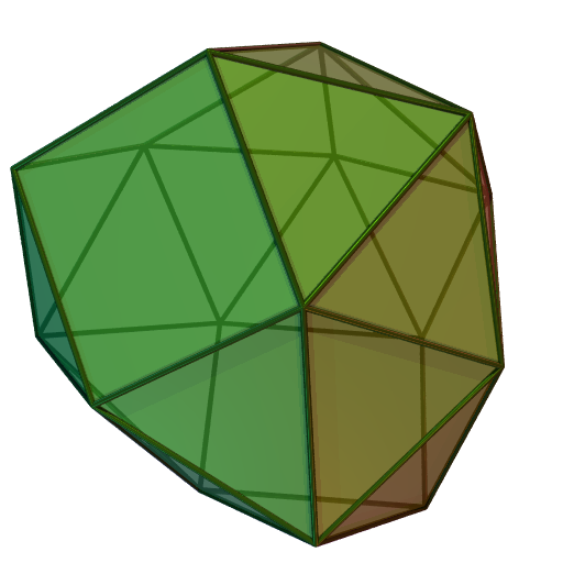
The Hilbert curve is meant to give you positions that, generally, are pretty close to one another. So if we take an image, say a disphenocingulum (which just happened to be 512x512 on wikimedia, and I have no idea what a disphenocingulum is ):

And we display is still as a 512x512 image, but this time the pixels follow the Hilbert curve as you go across each row, starting again at the beginning of the next row, then you get:


As you can see, it's definitely made the image, more, erm, horizontal. I was hoping that this could actually lead to improved compression for lossless formats like PNG and GIF. After experimenting with a few images, the 'Hilberted' images were always slightly bigger than the originals for PNG and slightly smaller than the originals for GIF (using PIL/Pillow for making the images).

Here's the size in kB for each method, for a collection of 512x512 PNG files found on the internet. The alpha channel, if there, was removed and set to black for each image beforehand:

Filename
Regular PNG
Hilberted PNG
Regular GIF
Hilberted GIF
002.png
64
89
78
62
android_sh.png
118
143
160
146
Disphenocingulum.png
91
104
165
154
edbang10.png
203
211
91
84
gear.png
107
122
114
95
imaso-512x512.png
253
272
156
140
iPhone 512x512.png
56
55
81
69
quiet 512x512.png
10
21
70
67
Todo-4-App-Icon-512.png
315
342
252
244

I think the reason for this is that GIF strictly encodes left-to-right and top-to-bottom, and in this case the 'Hilberted' versions do have more similarity left-to-right. However, PNGs have the ability to compare either the previous pixel to the left, or the pixel above (see here for details) or a combination of both. This simple approach to treating the data as 2d instead of 1d like GIF seems to really help with images with solid blocks of color, and although it's a lot simpler than the Hilbert method described above, it seems to produce better compression.

For GIFs, the Hilberted version is always slightly smaller (for the images tested). Note that for 5 out of the 9 images tested, the Hilberted GIF provided the smallest filesize out of all of the possibilities.

I'm including the code below. It needs the code above in a file called 'hilbert.py' to work. It has a variety of command line options for outputting processed and unprocessed images, and selecting the format to use. Hopefully they're documented well enough to make some sense.

The code for these two files can also be found on github.

# 2013-04-03 Trying Code && Beer at Substantial.
# what happens if we take the pixels in an image,
# rearrange using a hilbert curve, then save as png?
# is there any increase (or decrease) in compression
try:
    import Image  # needs PIL for this
except ImportError:
    from PIL import Image

import hilbert
import numpy as np
from StringIO import StringIO


def to_hilbert(im):
    im_dat = np.asarray(im)
    w, h = im.size

    if w & (w - 1) != 0 or h & (h - 1) != 0:
        print "Warning, dimensions", w, h, "not powers of two!"

    # let's create a new image for the transformed data
    imout = Image.new(im.mode, (w, h))
    imout_dat = imout.load()

    imout_dat_pos = 0
    for px in hilbert.hilbert(im_dat):
        imout_dat[imout_dat_pos % w, imout_dat_pos // w] = tuple(px)
        imout_dat_pos += 1
    return imout


def from_hilbert(im):
    w, h = im.size

    if w & (w - 1) != 0 or h & (h - 1) != 0:
        print "Warning, dimensions", w, h, "not powers of two!"

    # let's create a new image for the transformed data
    imout = Image.new(im.mode, (w, h))
    imout_dat = imout.load()

    imout_dat_pos = 0
    im_dat = im.load()
    # we create a matrix of x and y positions which we pass in
    xy = np.dstack(np.mgrid[0:h, 0:w])
    for (px, py) in hilbert.hilbert(xy):
        imout_dat[int(py), int(px)] = tuple(
            im_dat[imout_dat_pos % w, imout_dat_pos // w])
        imout_dat_pos += 1
    return imout


def to_image(im):
    w, h = im.size
    # let's create a new image for the transformed data
    imout = Image.new(im.mode, (w, h))
    imout_dat = imout.load()

    imout_dat_pos = 0
    for px in im.getdata():
        imout_dat[imout_dat_pos % w, imout_dat_pos // w] = tuple(px)
        imout_dat_pos += 1
    return imout


def test(file):
    im = Image.open(file)
    imout = to_image(im)
    assert(all(map(lambda (x, y): x == y, zip(im.getdata(), imout.getdata()))))
    imout = to_hilbert(im)
    imout = from_hilbert(imout)
    assert(all(map(lambda (x, y): x == y, zip(im.getdata(), imout.getdata()))))


if __name__ == '__main__':
    # we can test this on the 512x512 pngs in testpngs folder in bash with:
    # for f in testpngs/*; do python hilbert_png.py -t -f GIF -u "$f"; done;
    # this test, using GIF format, with unprocessing too 
    import argparse
    parser = argparse.ArgumentParser()
    parser.add_argument("file", help='The file to load')
    parser.add_argument(
        "--test", "-t", action='store_true',
        help="Doesn't write files, just calculates the sizes")
    parser.add_argument(
        "--reversehilbert", "-r", action='store_true',
        help="Reverses the effect of the program. Will restore the original image")
    parser.add_argument(
        "--unprocessed", "-u", action='store_true',
        help="Write an unprocessed file as well as a processed one.")
    parser.add_argument(
        "--outfile", "-o",
        help="File to write to.", default="out")
    parser.add_argument(
        "--unprocessedoutfile", "-uo",
        help="File to write unprocessed data to.")
    parser.add_argument(
        "--format", "-f",
        help="The format to use.", default="png")
    args = parser.parse_args()
    infile = args.file  # "out.png"
    im = Image.open(infile)
    # test("out.png")
    func = to_hilbert if not args.reversehilbert else from_hilbert
    if args.test:
        s = StringIO()
    else:
        ofile = args.outfile
        ofile += "." + args.format
        s = open(ofile, 'wb')

    imout = func(im)
    imout.save(s, format=args.format)
    if args.test:
        print "Size of hilberted %s %dKb" % (args.format, s.len / 1024)
    s.close()

    if args.unprocessed:
        if args.test:
            s = StringIO()
        else:
            ofile = args.unprocessedoutfile or 'unprocessed'+args.outfile
            ofile += "." + args.format
            s = open(ofile, 'wb')
        
        imout = to_image(im)
        imout.save(s, format=args.format)
        if args.test:
            print "Size of regular %s %dKb" % (args.format, s.len / 1024)
        s.close()


Monday, April 1, 2013

Hilbert curve in CFDG


Hilbert curve in CFDG

In a previous post, I talked about creating Koch snowflakes using the context-free design grammer (CFDG) program. In this post, I'll talk about how a Hilbert curve can also be created using a trick where the basic shape we use draws part of subsequent generations for us.

Hilbert curve is a little bit trickier (it was an xkcd comic that first introduced me to this fractal) than a Koch snowflake. The first generation looks like:
And the second generation looks like (I've included the first generation in gray on top of it):
The lines in green connect four copies of the first generation shape together. When we go to the third generation we can see four copies of the second generation connected here with red lines (with again the previous generations in gray):
So to create an nth generation Hilbert curve, we create four copies of the previous generation and connect them together with three additional lines. Unlike the Koch snowflake however, there's no single repeated shape, instead we need repeated previous generations plus connecting lines between them.

The upshot of all this is that there's no easy way to draw the nth generation of the Hilbert curve in CFDG (at least in the old version, it may be easier in the latest version) by repeating a simple shape, we need those extra connectors to join them up, and if we're trying to make it in a recursive fashion, there's no easy way to add them. 

If we look at the connectors we need (the green lines in the second generation, and the red lines in the third generation) we can see that they mirror the first generation shape somewhat - the three lines are in the same orientation, but are scaled and rotated. So if it's not possible to draw any generation with a simple shape, is it possible to draw all generations with a simple (although potentially recursive) shape? Can we come up with a shape which draws the connectors for subsequent generations?

The answer is yes. Take a look at the following CFDG code and it's output:
startshape H
 
shape H
{
 loop 2 [flip 90]
  iline[r 90   x -.5]
 iline [y -.5]
}

shape iline
{
 line[]
 iline [ s .5 y .25]
}

shape line
{
    SQUARE[s 1 0.01]
}
Hopefully this shape, when repeated, will give us all generations of the Hilbert curve (with each generation having some lines drawn by the previous generations). If we now repeat this shape four times scaled down by two, we get the following code:
startshape H
 
shape H
{
 loop 2 [flip 90]
  iline[r 90   x -.5]
 iline [y -.5]
 
 loop 2 [flip 90] {
  H [s .5 r 90 x -.5 y  .5]
  H [s .5      x -.5 y -.5]
 }
}
 

shape iline
{
 line[]
 iline [s .5 y .25 ]
}
shape line
{
    SQUARE[s 1 0.01]
}

And when we run this (and wait for 5 million shapes to be drawn) we get:


Which is exactly what we wanted. So here CFDG has allowed us to use a recursive starting shape, applied itself recursively to draw all generations of the Hilbert curve. There is no simple shape we could have used to create a single generation of the curve, and this approach draws all iterations, and must do as we draw the lines for future generations as we go along.

You can find my small collection of CFDG scripts here.

Thursday, March 28, 2013

Converting Grayscale to RGB with Numpy

Converting Grayscale to RGB with Numpy


There's a lot of scientific two-dimensional data out there, and if it's grayscale, sooner or later you need to convert it to RGB (or RGBA). I couldn't find any info about the bast way to do this in numpy, a typical scenario is converting a x by y array of floats into a x by y by 3 array of 8-bit ints. Numpy has a few ways to do it (that I could think of) and I figured testing them is the only real way to see which way's the fastest.
In the following, I'm assuming that any processing steps have already been taken, and all that's left is to truncate the values to unsigned 8-bit.

The file containing the tests can be downloaded from github.

Method 1: Basic

The first way I tried was to simply create the image and populate it with the array three times:

def to_rgb1(im):
    # I think this will be slow
    w, h = im.shape
    ret = np.empty((w, h, 3), dtype=np.uint8)
    ret[:, :, 0] = im
    ret[:, :, 1] = im
    ret[:, :, 2] = im
    return ret

This can be slightly modified (in Python, multiple assignment works by assigning the rightmost expression to all of the others, so the two methods here are different):

def to_rgb1a(im):
    # This should be fsater than 1, as we only
    # truncate to uint8 once (?)
    w, h = im.shape
    ret = np.empty((w, h, 3), dtype=np.uint8)
    ret[:, :, 2] =  ret[:, :, 1] =  ret[:, :, 0] =  im
    return ret

def to_rgb1b(im):
    # I would expect this to be identical to 1a
    w, h = im.shape
    ret = np.empty((w, h, 3), dtype=np.uint8)
    ret[:, :, 0] = im
    ret[:, :, 1] = ret[:, :, 2] = ret[:, :, 0]
    return ret

Method 2: Broadcasting


We can create the array as before, and assign it in one line, so I'd hoped this would be faster than method 1:

def to_rgb2(im):
    # as 1, but we use broadcasting in one line
    w, h = im.shape
    ret = np.empty((w, h, 3), dtype=np.uint8)
    ret[:, :, :] = im[:, :, np.newaxis]
    return ret

Method 3: Using dstack

The dstack method stacks arrays in the third dimesnion, and as the docs say 'This is a simple way to stack 2D arrays (images) into a single 3D array for processing'.

def to_rgb3(im):
    # we can use dstack and an array copy
    # this has to be slow, we create an array with
    # 3x the data we need and truncate afterwards
    return np.asarray(np.dstack((im, im, im)), dtype=np.uint8)


def to_rgb3a(im):
    # we can use the same array 3 times, converting to
    # uint8 first
    # this explicitly converts to np.uint8 once and is short
    return np.dstack([im.astype(np.uint8)] * 3)

But, there's a problem with the above: The returned array is not contiguous. This can be seen by comparing np.frombuffer(to_rgb3a(im)) vs np.frombuffer(to_rgb1(im)). Since most display code needs a contiguous buffer of RGB pixels this won't work. Luckily the copy function will fix this for us, but it requires an extra step:

def to_rgb3b(im):
    # as 3a, but we add an extra copy to contiguous 'C' order
    # data
    return np.dstack([im.astype(np.uint8)] * 3).copy(order='C')

Method 4: Using weave

Another way to do this is to use the weave module (included with SciPy) to write C code inline, which gets compiled to native code. Since many of the numpy functions are native code anyway it's not obvious this is going to make any difference, but it's something to try.

def to_rgb4(im):
    # we use weave to do the assignment in C code
    # this only gets compiled on the first call
    import scipy.weave as weave
    w, h = im.shape
    ret = np.empty((w, h, 3), dtype=np.uint8)
    code = """
    int impos=0;
    int retpos=0;
    for(int j=0; j<Nim[1]; j++)
    {
        for (int i=0; i<Nim[0]; i++)
        {
            unsigned char d=im[impos++];
            ret[retpos++] = d;
            ret[retpos++] = d;
            ret[retpos++] = d;
        }
    }
    """
    weave.inline(code, ["im", "ret"])
    return ret

Method 5: Using repeat

This was suggested by greger:

def to_rgb5(im):
    im.resize((im.shape[0], im.shape[1], 1))
    return np.repeat(im.astype(np.uint8), 3, 2)

Testing and timing

To test the above methods, I used inspection to find any functions beginning 'to_rgb' and tested them on data returned from the numpy.random.uniform function (which returns float64 data) for various image sizes, after checking all functions gave identical output.

The full code is here:

import numpy as np
import time
import sys


def to_rgb1(im):
    # I think this will be slow
    w, h = im.shape
    ret = np.empty((w, h, 3), dtype=np.uint8)
    ret[:, :, 0] = im
    ret[:, :, 1] = im
    ret[:, :, 2] = im
    return ret

def to_rgb1a(im):
    # This should be fsater than 1, as we only
    # truncate to uint8 once (?)
    w, h = im.shape
    ret = np.empty((w, h, 3), dtype=np.uint8)
    ret[:, :, 2] =  ret[:, :, 1] =  ret[:, :, 0] =  im
    return ret

def to_rgb1b(im):
    # I would expect this to be identical to 1a
    w, h = im.shape
    ret = np.empty((w, h, 3), dtype=np.uint8)
    ret[:, :, 0] = im
    ret[:, :, 1] = ret[:, :, 2] = ret[:, :, 0]
    return ret

def to_rgb2(im):
    # as 1, but we use broadcasting in one line
    w, h = im.shape
    ret = np.empty((w, h, 3), dtype=np.uint8)
    ret[:, :, :] = im[:, :, np.newaxis]
    return ret


def to_rgb3(im):
    # we can use dstack and an array copy
    # this has to be slow, we create an array with
    # 3x the data we need and truncate afterwards
    return np.asarray(np.dstack((im, im, im)), dtype=np.uint8)


def to_rgb3a(im):
    # we can use the same array 3 times, converting to
    # uint8 first
    # this explicitly converts to np.uint8 once and is short
    return np.dstack([im.astype(np.uint8)] * 3)


def to_rgb3b(im):
    # as 3a, but we add an extra copy to contiguous 'C' order
    # data
    return np.dstack([im.astype(np.uint8)] * 3).copy(order='C')


def to_rgb4(im):
    # we use weave to do the assignment in C code
    # this only gets compiled on the first call
    import scipy.weave as weave
    w, h = im.shape
    ret = np.empty((w, h, 3), dtype=np.uint8)
    code = """
    int impos=0;
    int retpos=0;
    for(int j=0; j<Nim[1]; j++)
    {
        for (int i=0; i<Nim[0]; i++)
        {
            unsigned char d=im[impos++];
            ret[retpos++] = d;
            ret[retpos++] = d;
            ret[retpos++] = d;
        }
    }
    """
    weave.inline(code, ["im", "ret"])
    return ret

def to_rgb5(im):
    im.resize((im.shape[0], im.shape[1], 1))
    return np.repeat(im.astype(np.uint8), 3, 2)

funcs = dict(((x,eval(x)) for x in list(globals()) if "to_rgb" in x))
print "testing Numpy v",np.version.version
print "on Python ", sys.version
for size in [64,256,1024,2048]:
    s = np.random.uniform(256, size=(size,size))
    op = [funcs[f](s) for f in funcs]
    assert(all(map(lambda x: np.array_equal(x, op[0]), op)))
    times=min(3*10**7/size**2, 10**5) or 1
    print "\n\nFor Size",size,"\n==============="
    for name, func in sorted(funcs.items()):
        start = time.time()
        for i in range(times):
            func(s)
        end=time.time()
        print "%s took \t%0.3f ms average for %d times" % (
            name, (1000*(end-start)/times),times)

Results

The results were a little bit unexpected, and highlight the idiom that testing is the only real way to gauge performance. The following table lists the average time in ms to process a 1024x1024 image. The Windows results were using a version of numpy compiled against MKL as found here. All results were from Python 2.7.3.

Architectureto_rgb1to_rgb1ato_rgb1bto_rgb2to_rgb3to_rgb3ato_rgb3bto_rgb4to_rgb5
MacBookPro
Win64/Python32
14.8 14.8 8.9 15.9 28.8 8.7 9.55.926.7
MacBookPro
Win64/Python64
3.3 3.2 4.7 6.8 17.4 3.8 4.83.721.1
MacBookPro
OSX64/Python32
2.6 2.6 3.7 9.2 20.1 2.9 3.41.419.9
MacBookPro
OSX64/Python64
2.7 2.6 3.6 5.7 16.7 2.8 4.12.118.4
Xeon W3520
Win64/Python32
9.2 9.2 8.4 22.4 54.1 12.3 40.36.8
Xeon W3520
Win64/Python64
5.7 5.3 7.2 13.7 51.3 10.9 30.04.4

The first thing to notice is just how varied these different methods are. to_rgb3 is the only obviously sub-optimal implementation, and it shows, being the slowest for any configuration. There is a surprising difference in the performance under Windows 7 vs MacOSX for the same hardware, with the Mac performing noticeably better. to_rgb3a works well under most configurations, but the overhead of the extra copy in rgb_3b varies from being relatively minor (~10% for Win64/Python32) to awful (~200% for the Xeon Win64/Python64).  The Python32 results under Win64 are awful for the MacBook, but relatively better for the Xeon machine.

1 and 1a produced identical results, with 1b working noticeably better under Win64/Python32 but worse in the other configurations.  Method 2 was surprisingly slow, especially considering it was one call into C code.

In general the results above are just confusing, and vary significantly on different platforms and different architectures. Methods 1/1a give generally decent results, and I can't think of a good reason not to recommend them, so I'd have to go with 1a as the least worst most generally optimal solution, and the one I'd tentatively recommend. The weave results are generally good, but they do require a compiler to be installed and set up on the machine in use. Another thing to note is that converting to 8-bit doesn't coerce values, so you need to be careful to do this yourself if needed. In this case using weave to coerce and assign all at once may well give the best performance.